3D Reconstruction: TSDF Fusion and Marching Cubes

Overview

The world we live in is 3D in nature. Just about every object a typical human physically interacts with is 3-dimensional in nature. However, when engaging in our favourite pastimes of media consumption we are limited to 2D (or at best, faux 3D).

From movies to video games, we consume media on flat screens, relying on our imagination to upsample it to 3D. For example, this video of me circling a Zoro figurine is in 2D ¹. Our minds can pretty easily interpret this as a 3D figure. Go ahead, rotate Zoro upside down in your head.

Figure 1: A cookie for you if you flipped him. 🍪

Representing 2D media in its true 3-dimensional glory is a long-standing and fundamental problem in Computer Vision and spans several decades of research. Needless to say, the problem of 3D Reconstruction is a vast one with many different variants and solutions.

In this post we tackle 3D Reconstruction in the following setting:

Given a sequence of depth images and camera parameters, recover a 3D mesh of the captured scene. The environment is assumed to be rigid (i.e. nothing moves except the camera.)

Specifically, we will make use of the TSDF Fusion and the Marching Cubes algorithms to generate the 3D mesh.

The Algorithm

The inputs:

• Depth: A depth image is simply a measure of of how far each pixel of the image is from the camera. With recent advances in CV, can be computed well even from a single image!

• Camera Parameters: The camera parameters describe the properties of the camera. Typically, this consists of the intrinsic (how the camera maps the world to an image) and extrinsic (where the camera is in the world) matrices.

TSDF Fusion

Almost 30 years old, the seminal paper by Curless and Levoy describes a method to integrate sequences of depth images into a 3D volume incrementally and extract a mesh. The various properties of the algorithm (parallelizability, incremental updates, control over speed/accuracy) makes it a popular choice for all sorts of applications from robotics to augmented reality.

The core idea of the algorithm is to maintain a 3D volume (voxel grid) where each voxel stores a TSDF value. The Truncated Signed Distance Function (despite the somewhat intimidating name) is simple. The Signed Distance Function (SDF) at a point is the distance of the nearest surface from the point. If positive, the point is in front of the surface, if negative it is behind and when the SDF is 0, the point is on the surface. For optimization purposes, the signed distance function is truncated, i.e voxels with a SDF value greater than a threshold are ignored.

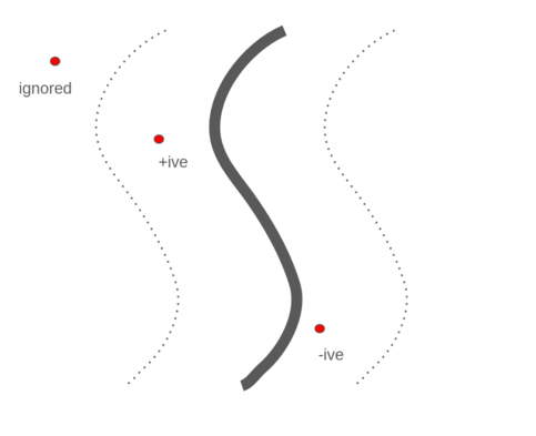
Figure 2: A very simple illustration of the TSDF function, positive “in front”, negative behind and ignored if too far from the surface.

To calculate the SDF of a voxel, we need to first project the voxel to the image plane and then compare with the sensor depth at that pixel location. An example to illustrate:

Consider a voxel $(x,y,z)$ at $(10,10,10)$ and camera focal length $f = 5$. Using the pinhole camera model, we project the voxel coordinates $(x,y,z)$ to the image plane $(u,v)$:

With $u = 5, v = 5$ Now let’s say the depth sensor records a value of $d = 9.9$m at the pixel coordinates $(5,5)$. Then the SDF of the voxel is calculated as:

And then TSDF is calculated as ²:

Typically, the TSDF is normalized by the truncation threshold $\tau$ for numerical stability and optimization purposes. Assuming a threshold $ \tau = 0.2 $, our TSDF value is $ TSDF_1 = 0.5 $. This describes the simple case of one voxel, one depth pixel and one camera pose. Now consider that the sensor is placed at another location (i.e. different camera pose), and the new TSDF measurement at that voxel is $ TSDF_2 = 0.3 $.

To fuse this measurement into the TSDF volume, we have the core of the algorithm, the TSDF update equation:

Where $TSDF_{k}$ represents the current cumulative TSDF value at the voxel and the incoming measurement by $ \text{tsdf}_{k+1}$.

Similarly $W_{k}$ represents the cumulative weight at the voxel and ${w_{k+1}}$, the incoming weight. The weights are used to control the impact of the new measurement. In the simplest case, this could be set to 1, resulting in an averaging out of TSDF over time as $W_k$ gets larger and larger. Alternatively, this could be the confidence of the depth measured by your sensor.

In our toy example, assuming $TSDF_k = 0.5$, $W_k = 1$, $tsdf_{k+1} = 0.3$ and $w_{k+1} = 1$, we have:

This weighted update mechanism from different camera locations averages out the errors in the depth and the camera pose, providing a smooth output mesh. We’ve looked at fusing multiple depth values for a single voxel. Extending the algorithm to its general form is fundamentally the same.

Given a sequence of length $N$ containing depth and camera poses $D_i, P_i$ for $i \in N$ and the camera intrinsics matrix $K$, the TSDF fusion algorithm is described as follows:

1. Initialize the TSDF volume
2. Sequentially feed in a pair of depth/camera pose - $D_i, P_i$
3. Project the volume to the image plane (use camera pose $P_i$ and intrinsics $K$)
4. Calculate the new TSDF values using $D_i$
5. Update the TSDF volume
6. Repeat steps 3-5 until all images are processed.

Marching Cubes

We have our final TSDF volume, a voxel grid where each voxel contains the distance to the nearest surface. Now what?

Enter Marching Cubes - an algorithm for extracting the mesh of an isosurface from a voxel volume. The isosurface ³ represents the surface that contains points of a constant value. In the case of our TSDF volume, the constant value is 0, which indicates points that are on the surface of the mesh.

The algorithm itself is straightforward. It operates independently (“marches”) on each voxel (“cube”), generating the mesh for that particular voxel. Consider a TSDF volume of resolution $N^3$. Marching cubes operates inside this volume, where each of the 8 vertices of the cube hold TSDF values. There are $(N-1)^3$ cubes.

Every vertex has two possibilities, the TSDF can either be $>0$ (vertex outside surface) or $<0$ (inside surface). We have 8 such vertices, and it follows that every cube belongs to one of $2^8 = 256$ configurations. The idea behind Marching Cubes is that each of these 256 configurations maps to a particular combination of edges and triangles, and we can simply look-up the triangles of the mesh for this configuration. The TSDF magnitude at the vertices allow us to refine where exactly inside the cube the triangles need to be placed. Fortunately, due to symmetries in the cube, these 256 configurations can be simplified to just 15 cases ⁴, as seen in the below figure from the original 1987 paper.

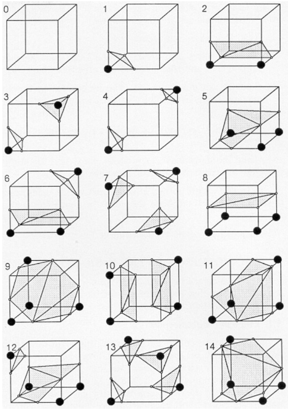
Figure 3: Various patterns of points within/outside the surface and the corresponding triangulations.

And …. that’s it! Every cube generates a piece of the mesh, and put together, we have a complete 3D mesh! To really get down to the nitty gritty details, let us progress towards the code.

Implementation

Depth and Pose were obtained using COLMAP. Code was implemented in numpy. Depth and pose not to scale, not in metre. rgb/d image -> ooh that cool drag and visualize 2 in one thing.

Hyperparameters to care about. Snippets to care about (with syntax highlighting) and explanation.

tsdf volume visualization.

final - display coloured zoro mesh interactive - three.js

Extensions

Voxel Hashing Dual Contouring monocular image neural monocular video neural - neuralrecon nerfs / gaussian splatting

References

• An implementation of TSDF Fusion by Kevin Zakka
• JustusThies/PyMarchingCubes
• A Volumetric Method for Building Complex Models from Range Images - Curless and Levoy
• KinectFusion: Real-Time Dense Surface Mapping and Tracking
• VDBFusion: Flexible and Efficient TSDF Integration of Range Sensor Data
• Real-time 3D Reconstruction at Scale using Voxel Hashing
• Marching cubes: A high resolution 3D surface construction algorithm
• A survey of the marching cubes algorithm

Footnotes